Week 12 Georeferencing, Editing & ArcScene

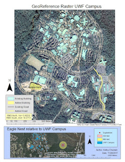
This week I was provided shape files of the buildings and roads on UWF campus that had been geographically referenced coordinate data built in to the files (as has been the other files provided so far).  Also proved, two aerial raster files of UWF campus with no referenced coordinate data built in.  "Through a process called georeferencing, also called 'image registration', I tell the raster dataset 'where it belongs'.  This is done by identifying a common point on the target layer and an already referenced control layer and linking these common points."  Since this is a new task, I needed to add the georeferencing toolbar (right click any unoccupied area in the grey area around the toolbars and check georeferencing to add that toolbar).  To make the images line up I add control points (clicking that icon from the georeferencing tool bar), clicking first the point on the unknown (raster-aerial) and then the same point on the known (vector - building or road).  For best results the points should be spread out not clustered together or in strait lines.  Can be tricky accessing points with all of the files in the same window you can either set either the referenced or the unreferenced layer to a transparency (layer properties, display) or a new viewer window (icon in the GeoRef. toolbar) that only displays the raster (this was my choice).  When you aren't satisfied the delete the link with another icon on the GeoRef toolbar.  After 5 points review the links with the 'view links table' icon.  Residual value shows how much each link agrees with how the layer is currently being displayed.  The lower the residual value the more accurately that control point is georeferenced.  Root Mean Square (RMS) is used to indicate the accuracy of the spatial analysis.  The lab pdf indicates the RMS should remain under 15 with 10 control points.  Mine was 5.08232 (so I thought I was an expert!), until the second aerial was added and control points were added.  This photo was intentionally distorted - HOW RUDE!  I was able to get the RMS VERY low with a 3rd Order Polynomial but the map appearance was not matching up well with non control points.  At a 2nd Order Polynomial is the RMS was 14.2713, but the map looked more matched up overall.  "Higher order transformations allow the raster to bend and warp more than lower order transformations."  Update georeferencing (in the georeferencing drop down) to finish.

Next I edited the referenced image by adding a building and a road not in the original building and road files.  Again a new task means adding a new toolbar.  This time click Editor Toolbar icon on the standard toolbar to display.  To begin in Editor Toolbar drop down "start editing".  Select the layer to which the edits will be made from the TOC.  Select "Create Feature" icon confirm the feature template and select the construction tool in the create features window.  Set up additional editing properties like snapping.  Select the strait segment icon and start adding vertex. (End point arc was also suggested along with the strait segment icon, I did not use it).  Add vertex to keep the shape.  Double click vertex to end.   Save edits (this is not saved in the map until this selection) end editing session in the Editing tool drop down.

Next a multiple ring buffer was requested to a point file provided marking an Eagles Nest.  A hyperlink was directed in the attribute table to a photo of this nest (attribute table icon in the editing toolbar).  Add Multiple Ring Buffer tool icon (Customize (main menu-Customize Mode-Commands tab-search Multiple Ring Buffer-click and drag to empty spot on toolbar area).  Multiple Ring Buffer tool window requires input, output, buffer unit, and distances).  This point is not contained in the aerial files provided.  After the buffer was performed a base map was added to show the general location of the nest in relation to the UWF campus buildings.  The protection buffer was set to 50% transparent.  Here is the map!!

Finally this week create a 3D scene in ArcScene.  This was the briefest of introductions.  I opened ArcScene (start-ArcGIS-ArcScene).  Added the same layers; buildings, roads, aerials.  Attempted to more around with navigate and fly icons.  I opened the property of each layer and in base heights tab selected "floating on a custom surface (from UWF_DEM).  I added a layer offset of .1 to the base heights tab of the north aerial to get rid of a black line between the north and south aerials.   In the properties of the building layer in the extrusion tab check extrude features in layer, typed "Height" into the expression box, and in apply extrusion by  selected adding it to each features maximum height.   From the main menu View Scene Properties, general tab, changed vertical exaggeration to 5.  Here is that map!

Week 11: Geodocding, Network Analyst & Model Builder

First on the list this week:  1)geocode Emergency Management Service sites for Lake County, FL (addresses from LakeEMS.org).  Utilized US Census Bureau Tiger line files after downloading and projecting.  Set up and address locator.  Utilized table provided with addresses of the locations for Lake County, FL EMS locations to geocode (tie an address to a place in the map).  Then researched using Bing maps, the source web site LakeEMS.org to locate those unmatched locations and either selected a candidate from the interactive rematch window or manually placed locations.


Next this week 2)Network Analyst: utilize Arc GIS extension Network Analyst to create a simple route map output.  Utilized Network Analyst (customize-extensions-network analyst) to add stops.  In the Route properties window (layer properties) from the network analyst window I specified route to be calculated based on travel time in minutes based on a specific day and time.  Clicked the solve button from the network analyst toolbar.  Looked at the Directions window from the network analyst tool bar.  Saved as mxd.  Here is my map with the EMS locations, Lake County boundary, Streets layer, and the optimal route showing my 3 stops.

Lastly this week 3)explored simple model in Model Builder.  This exercise was completed in ESRI Virtual Campus.  Performed edits to an existing model.  Input=Blue Oval, Rectangle=Tool, Output=Green Oval.  Not sure if the colors and shapes are universal for all models or specific to this one.  This model created buffers, performed an intersect of the buffers and final dissolved borders of the intersect to create polygons.  Here is a screen shot of the model (looks like flow chart!)

Week 10: Spatial Analysis (week 2)

This week the map assignment was to utilize shape files to find potential camp sites that are within 300 Meters of a road, 150 Meters of a Lake, 500 Meters of a River and outside of any conservation area.  First to buffer the road shape file: Arc Tool Box button, Analysis Tools, Proximity, Buffer, 300 Meters and dissolve (overlapping buffer edges are removed).  Next to buffer the water feature class took a few more steps.  Separate buffers of 150 Meters for lakes and 500 Meters for rivers.  Insert field to the attribute table for the water feature class and name the field buffdist (for buffer distance), right click the new column heading and select field calculator and define the buffers for lakes and then "switch selection" button and define for rivers.  Next my first experience with ArcPy (is a Python site package for performing geographic information system (GIS) functions available in ArcGIS).  That's right Python, as in programing language!  I wrote my first script and practiced inputting multiple scripts to run simultaneously.  Next I had to get the water buffer and road buffer together.  The lab assigned a Union Overlay and then to export (TOC-Data-Export Data - Selected Features) to a new feature class.  Then to do another overlay that would result in the same outcome, I chose an Intersect Overlay.  For this exercise, I found no noticeable difference in the outcomes of the Intersect Overlay and the Union Overlay.  Then I needed to exclude any conservation areas from my results of possible camp sites.  I chose to use Erase Overlay, to remove conservation areas from my results.  Next I changed the multi-part layer (only 4 records in the attribute table) to a single-part layer (allowing more specific feature selection).  Back to the Arc Tool Box-Data Management-Features-Multipart to Single part.  Finally adding a field to the single part attribute table for area and utilizing calculate geometry option for the math to be preformed.  It didn't really feel like a lot this week, but writing it all out sure makes it sound like a lot.  Here is my final map!