Module 10: Supervised Classification

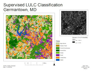
This week we continued to look at automated classifications, focusing on Supervised Classifications.  Supervised Classification requires the user to set "training sets" to guide in the separation of the pixels into classes.  The objective of the training sets is to select a homogeneous area for each spectral class.  Selection of multiple training sets helps to identify the many possible spectral classes in each information class of interest.  Training sets can be selected by 1)digitize polygons, that have a high degree of user control but often result in overestimate of spectral class and 2)seed pixel where the user sets thresholds.  Both of these methods were utilized this week in lab.  Training aids help evaluate spectral class separability, for example graphical plots like histograms, coincident spectral mean plots, or scatter plots.  There are also statistical measures of separability like divergence or Mahalanobis distance.  Parametric distance approaches are based on statistical parameters assuming normal distribution of the clusters (mean, std deviation, co-variance).  Examples of parametric methods are mahalanobis distance, minimum distance and maximum likelihood.  Non-Parametric distance approaches are not based on statistics but on discrete objects and simple spectral distance (examples are feature space and parallel-piped).

In lab this week we produced classified images from satellite data.  We created spectral signatures and areas of interest (AOI) features utilizing both digitize polygons and seed pixels.  We evaluated signatures by with histogram plots and mean plots to recognize and limit spectral confusion between spectral signatures.  We classified images utilizing maximum likelihood classification and then merged classes and calculated area.

Module 9: Image Classification

This week we continued with image classification.  Image Classification is a major application of remotely sensed imagery to provide information on land use and land cover.  In a previous weeks we utilized tone, texture, shape, size, pattern, shadow and surroundings to identify and classify.  Then moved on to looking at different spectral bands.  This week we move toward automated procedures.  Spectral Pattern Recognition is a numerical process whereby elements of multispectral image data sets are categorized into a limited number of spectrally separable, discrete classes.  Unsupervised Classification, the focus this week, uses some form of clustering algorithm to decide which land cover type each pixel most looks like.  Supervised Classification, next week, uses training sites from multiple spectral band data to guide the computer's classification.   

Tools like Feature Space Image allows visualization of 2 bands of image data simultaneously through a 2 band scatterplot, one band plotted on the X and the other on the Y axis.  This tool helps consider covariance, correlation and clustering between bands.  Spectral Distance, is one means of predicting the likelihood that a pixel belongs to one class or another.  Spectral Distance can be measured as simple euclidean distance in unsupervised or a statistical distance in supervised.  These tools help to differentiate spectral classes, clusters of spectrally similar pixels, that can then be used to form information classes, meaningful groups.  

This week in lab we performed unsupervised classification in both ArcMap and ERDAS.  We attempted to accurately classify images of different spatial and spectral resolutions.  And we manually reclassified and recoded images to simplify the data.  We utilized ISODATA (Iterative Self-Organizing Data Analysis Technique) Clustering Algorithm.  

The map this week is of the UWF campus.  The main map was created by utilizing ISODATA classification in ERDAS.  The tool was set to 50 classes with 25 iterations with a convergence threshold of 0.95 and a skip factor of 2 for both X & Y.  Reclassification of the 50 classes to 5:  trees, grass, building&roads, shadows and mix.  The reclassification was then merged into the 5 classes.  The lab instructions were to calculate an estimate of porous and non-porous surfaces in the image.  I decided to run ISODATA with the same specifications and reclass based on porous, non-porous, and mixed.  Both processes proved difficult primarily due to pixels categorized in the same groups of 50 that were different information classes.  Pixels for roads, parking lots and roof tops sharing groupings with grass or bare ground.   With the original 50 classes to ulizmarly get 5 classes for the main map and 3 classes for the insert the error ratio, based only on my opinion of the visual inspection, is still high.