Scale Effect & Spatial Data Aggregation

Scale effects on vector data seem to be intuitive.  When you taking real earth and shrinking it down to fit on a page there will be details that will be lost or moved or changed.  Does your map scale allow for rivers, how about major creeks, does it show smaller tributaries?  The details that are not the focus are often eliminated the details that are the focus maybe included but require shifting of other features to get them to fit.

Resolution effects on raster data are also intuitive.  This is easiest demonstrated by a discussion of pixel.  The high the number of pixel for a photo the larger the picture can be made without looking blurry.  Raster data is contained in grids of cells.  At smaller cell size, 1m or 2m,  the more detail is available.  As the cell size gets to be larger (10m, 30m, 90m) the sample data is averaged in those cells.  The creates smoother data as the highs and lows are lost in the averaging.  And the imagery becomes more pixelated at finer resolution.

Modifiable Area Unit Problem (MAUP) exists for aggregation and zonation. Just because there are more area units does not mean the data is more specific and granular.  I can combine several areas to make larger areas and then put many many small areas into the mix.  I may end with more areas, but less detail than a lower number of evenly distributed area units.

Gerrymandering refers to odd shapes that can arise in political districts when the boundaries are manipulated for statistical properties.  Include this set of people and exclude those and we can raise or lower all kinds of statistics.  Determining the Polsby-Popper score results in a range 0-1.  The closer to 1 the more compact a polygon.  Polsby-Popper was calculated as 4*pie*area / perimeter^.  Below in red are the top 5 Congressional Districts in the Continental US that have lowest compact score, indicating the highest probability of gerrymandering.

Surfaces - Accuracy in DEMs

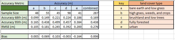
This week we examined vertical accuracy of DEMs.  We were provided with a raster file of high resolution bare earth DEM obtained through LIDAR and and excel file with field observations of ground elevation.  The field data contained 5 land cover types (a-e).  We utilized the Extract Multi Values to Points tool.  This tool grabs the elevation value of the pixel of the lidar raster directly beneath each sample point.  We added a field to the attribute table to convert feet to meters.  Accuracy was calculated for each land cover type and then the all the data combined.  We summarized the comparison in the table above.  The calculations in the table are the differences in meters from the DEM to the reference field data at 68%, 95%, RMSE, and Bias.

RMSE

• difference between DEM and reference for each point
• Square the difference for each point
• Average the squared differences (Sum the square difference/count of points)
• Square root of the average 

Bias as ME - is the average of the errors

Interpolation

 This week we carried out different surface interpolation techniques.  To the right you will see:

1)IDW:  Inverse Distance Weighting.  This was performed with IDW tool.  Generally the process takes the known sample points and infers values at other points.  This is accomplished by taking the known values and assuming areas in proximity of this will have similar results.

 2)Spline Interpolation Regularized: This method utilizes minimum curvature to fit boundary divisions through and around sample values.  I imagine laying out a piece of yard around the data values to form the boundaries for classifications.

3) Spline Interpolation Tension:  This method again utilizes minimum curvature to fit boundary divisions through the sample values.  Tension setting causes the barrier lines to be a bit more stiff, displaying as less fluid.

TINs and Dems

This week we moved from data quality to started looking at surface information.  We created 3d visualizations of elevation models, and examined TINs and DEMs.   

TIN, Triangular Irregular Network, is a vector display of triangles formed between elevation points the sides or edges of the triangles cover the study area without overlap or gaps to interpolate changes in elevation over distance to provide estimates of slope. Displayed above is a TIN.  The triangular network is visible with graduated color of slope and contour lines with darker index contours.

DEM, Digital Elevation Model, utilizes raster data stored in the raster cells.  The cell data is processed utilizing a model like nearest neighbor, 8 cell window, or other to provide elevation data.

Data Quality-Standards

This week in class we examined the accuracy of two road networks, Street Map and City of Albuquerque.  We calculated accuracy with procedures provided by the National Standard for Spatial Data Accuracy (NSSDA).  We selected 20 street intersection locations and marked the location of the intersection provided in the Street Map data as well as the same intersection location for the City data.  We referenced each of these data sets with ortho-rectified imagery.  The test points are shown above in green for the city data, red for the street map and blue (slightly larger symbol) for the reference.  Finding appropriate test points was more challenging that I initially thought.  20 minimum points, with a minimum of 20% in each quadrant with minimum separation between points of 10% of the diagonal of the study area.

Accuracy Statistics were calculated seperately for City data and Street Map each utilizing the Ortho points as the reference.  The XY data of each point was obtained in ArcPro.  Those points were exported to Excel.  The calculations included differences for X & Y coordinates, each difference squared, and then the sum of X & Y.  Those sets were summarized as Sum, Average, RMSE, and NSSDA.

Formal accuracy statements as per the NSSDA guidelines are:

Horizontal positional accuracy for Street Map:  Tested 70,116.2 Feet horizontal accuracy at 95% confidence level.

Horizontal positional accuracy for City of Albuquerque: Tested 605.8 Feet horizontal accuracy at 95% confidence level.

 
The accuracy position at 95% confidence is quite different:  City data at 605.8 feet; Street Map at 70,116.2 feet.  The importance of knowing the source of your data as well as its accuracy became abundantly apparent! 

Calculating Metrics for Spatial Data Quality

Horizontal Precision @68% 5.65meters

Vertical Precision @68% = 5.71meters

Horizontal Accuracy from the average point is 5.82 meters

Vertical Accuracy from the average point is 5.96 meters

Week one of Special Topics:  Learning Outcomes 1)understand the difference between precision and accuracy 2) calculate vertical and horizontal position accuracy and precision 3) calculate root-mean-square error (RMSE) and cumulative distribution function (CDF).

What is the difference between Accuracy and Precision?  Our text reports "Positional accuracy measures how close a representation of an object is to the true value." (Bolstad, 2017, p. 264).  And "Precision refers to the consistency of a measurement method." (Bostad, 2017, p. 264).  Another source describes it as "The accuracy of a measurement means getting a value that is close to the actual answer. Precision, on the other hand, refers to the reproducibility of this result that is you get the same result every time you try." (Nedha, 2015, para 1).  So precision is the repeatability of the results, and accuracy is how close to the referenced point (actual location).  

Precision for this lab was measured by calculating the % of precision desired (common is 68%) of the total sample points.  Sorting sample points from lowest to highest values and utilizing the measurements of the nth(68% of 50 sample is 34) sample.

Accuracy for this lab was measured by calculating the average of all sample points and comparing it to the referenced/actual point.

Reference:

Bolstad, P. (2017). Gis fundamentals: a first text on geographic information systems. Acton, MA: XanEdu.

Nedha. (2015, July 13). Difference Between Accuracy and Precision. Retrieved from https://www.differencebetween.com/difference-between-accuracy-and-vs-precision/