Module 5a - Intro to ERDAS Imagine & Digital Data

This week in lecture we learned about Electromagnetic Radiation (EMR), models of EMR focusing on the Wave model, Electromagnetic Spectrum, EMR interactions of refraction, scattering, absorption, reflectance and transmission.

In lab this week we were exposed to ERDAS Imagine for the first time.  We used basic tools to add data, fit to frame, adjust vector symbology, navigate the image, set default data directory and default output directory, and changed band combinations to examine enhancements.  The project we added an area column in the attribute table in ERDAS, selected a small area of image utilizing the inquire box and created a subset of the image from the inquire box and saved to output as .img.  The .img was opened in Arc Pro and the above map created to show the classes within my subset and the area of each of classes.

Module 4: Ground Truthing and Accuracy Assessment

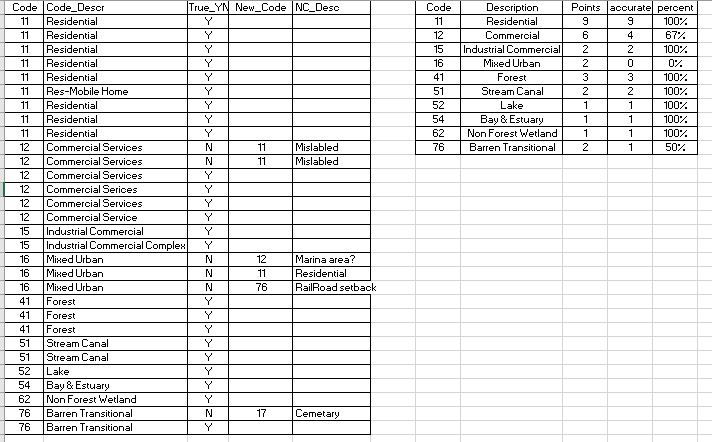
This week in lab we took our LULC map from last week and performed ground truth via Google Map.  I randomly selected 30 points in a grid fashion and then adjusted to account for each land type from the original map.  Each point was located and verified in google map for the location land use.  Here is a summary table of those results.

Of the 30 sample points 24 of them were classified correctly for an overall accuracy of 80%.  The smaller table above shows the accuracy broken out by classifications.  Mixed Urban had 0% correct.  Since I utilized this class for areas that I could not completely identify when classifying it is reasonable that with additional data the need for this classification would be eliminated.

Land Use Land Cover Classification

This week in lab we practiced our skills of recognizing features on the ground using a natural color aerial photograph.  We digitized an area of Pascagoula, MS, creating a land use/land cover map.  We identified the ground based on size, shape, color, pattern, shadows and association.  We utilized the USGS Standard Land Use / Land Cover Classification System.  The assignment was to categorize to level two (two digit classification).  Classifications of three or higher are typically utilized for local and some regional planning. 

My specific categories for this project 

Part of my employment background was working for 10 years in a building department in a municipality.  We worked very closely with the planning department and GIS guy.  Identifying urban land use from aerial perspectives I have done before.  It is a lot easier when you are familiar with the area.  Correctly identifying natural elements just at a level 2 classification was difficult because I am not familiar with the difference in kinds of trees or when a stream or canal becomes part of an estuary or bay. 

Technically doing the polygons was new and still somewhat challenging in the new to me GIS Pro.  My first attempt I did not have the Edge snapping or vertex snapping turned on, so I utilized this attempt as practice.  The second attempt I did turn on the snapping features while creating the polygons.  First creating a feature class file in my gdb.  Then in the edit tab clicking the create button and choosing polygon.  It was challenging to be able to navigate the picture while creating the polygon.  I settled on zooming in and out with the mouse scroll to move the image without having to click.  I did not master the clip portion to separate smaller interior polygons from larger surrounding areas.  Instead I relied on more of a lasso method with the larger polygon.  I started with larger easily identified areas keeping my attribute table open and adding the code as I drew each polygon (realizing that you must click off the cell in the attribute table that you are making changes to before you save the changes or that cell will not be recorded).  As I progressed from larger isolated polygons then I started working right and left back and forth to fill in the surrounding areas and smaller isolations.  Distinguishing between commercial service and commercial industrial was harder without knowledge of the practice of the location.  Ultimately, I settled on cleaner sites without outside materials or industrial roof or ground mechanisms and Commercial Service and those with as Commercial Industrial.

Visual Interpretation

This week in Photo Interpretation and Remote Sensing we  learned more about the types of and techniques for interpreting aerial photography. We were provided background on the types of aerial cameras, the different types of images they capture (oblique, vertical, stereo), the types of film used by traditional cameras, and understand how resolution (spatial, spectral, temporal) applies to aerial photography. We also learned concepts, techniques, and application of visually interpreting aerial photos. We learned about the methods and techniques used to visually interpret aerial photos (i.e. recognition elements). These techniques form the basis for deriving geographic features and/or land use land cover types from aerial photos and that are used in a wide variety of real world applications. 

In the laboratory exercise, we learned some basic principles of interpreting features found on aerial photographs.  The first map above illustrates ranges of tone and texture for this photo.  The second map above demonstrates examples of elements identified, at least partially, by shape and size, pattern, shadow, and association of the surroundings.  We also examined a true color image (blue, green, red), identifying 5 areas of color and compared those elements in the same image provided in false color (green, red, and infrared).

We have moved from ArcGIS desktop to ArcGIS Pro and it has been a disorienting week.  The changes are vast! location of symbology, labeling, and properties are different, but even the environment has changed to a project oriented system instead of .mdx maps.  I am sure I will catch up as soon as I figure out how to control drive location.  

Final Project: Plano, Texas Exploration

Project Proposal:  Plano, Texas Exploration for Hobbs’

 My final project is a location decision for Mr. and Mrs. Hobbs.  They moved to Plano, TX to retire in April to be closer to their daughter and her family.  They are unfamiliar with the area and have asked me, another daughter, to come up with some geographic information for them.  They have already found their new home but would like to get to know the area better.  They asked for locations of the hospitals, parks, airports, toll roads and any other information that would assist them in becoming acquainted to their new environment.  Locating amenities near the Hobbs’ will provide them with a much clearer picture of the area and help them feel more at home.  Maps and tables are provided to highlight areas like their home in relation to their daughters and the location of the toll roads, hospitals and airports.  Geocoding of farmers markets, museums and other destinations have been included.  GIS analysis of buffered and clipped data to utilize for euclidean distance and weighted overlay analysis has been performed to come up with some areas for the Hobbs' to explore based on their interests.

Final Project: Python

My final project proposal is to locate cities or towns in Texas of a minimum size (thinking 100,000) that are within 50 miles of a major airport that contain a lake or river.  I will need to obtain data for the state of Texas including lakes and rivers as well as airports and population of cities.  Utilizing python script: 1) create a buffer around airports of maybe 50 miles.  2)Clip population data and lake/river data to airport buffers.  3)utilize the results to Create a search cursor to locate cities or towns over 100,000 in population 4)print the list of locations.

First image above is of the printed list of cities/towns with populations over 100,000, that are within 50 miles of an airport and the second is of the printed dictionary containing the name of the city and the population.  Below is an image of the catalog files showing the Clipped cities and NHD in the results folder.

Module 11: Sharing Tools

The FINAL MODULE for GIS Programming!  We explored different methods for sharing script tools, learned ESRI recommended folder and file structure for sharing script tools, identified data and workspaces for script tools.  We learned  how to created a geoprocessing package, embed scripts and password protection tools and created script tool documentation.

This week in lab we focused on the standard folder structure and filepaths necessary when sharing tools and looked at some geoprocessing packages that provide an alternative solution to distributing script tools.

Module 10: Creating Custom Tools

This week we created a custom tool.  We were provided with a stand alone python script.  In ArcMap we created a toolbox and added the script to the toolbox (adding a description and check the "store relative path names").  We added parameters to the tool by right clicking the tool and choosing parameters 1.  Input file location 2. Clip Boundary Feature 3. Input features 4. Output file location.  We set the types for each and location:

Proposal Final Project

This week we prepared our Final Project proposals.  We were provided with a template that outlined sections (Title, Introduction, Methods, Anticipated Results, References) and specifications that were to be addressed in each section.  The proposal written using clear, specific, professional and descriptive language in word format.

I am planning to relocate to this area in the future.  My sister is in Murphy and my parents just relocated to Plano in April.  I wanted to do my project on this area to gain some information for myself of the area.  Initially I thought of looking at the surrounding counties to see some of their economics and natural resources to find areas I might want to focus job searches.

This project made several transformations as the realization that my original desired study area (Collin and surrounding counties) was recognized as much too large.  Another revision when the data that I had acquired for the large area wasn't translating into a smaller study area (airports, lakes and geographic named areas are mostly outside of the study area).  Further revision when I realized that Plano and Murphy are so disproportionate in size, that comparisons were unrealistic.  Finally settling on this Exploration of Plano Texas.  As my parents have only recently moved here, focusing the project on finding and displaying data that would be useful to them, assist me with learning about the area (although limited) and a focus for this school project.

The base map above includes boundaries, roads, railroads, the lone airport, parks and surface water.  The concern for the location of toll roads is already being addressed in the base map and will continue to be highlighted by the bold symbology.  The goal of the project will be to include layers to the parks and water features for farmers markets, destinations and museums.  This will provide visual reference for where to go to do something fun.  A more informational map showing locations of hospitals in the area.  Maybe a larger scale map to show the locations of the airports.  An even larger scale map to show the names of surrounding counties to better follow weather alerts in their area.

Module 9: Raster

This week we learned how to use Python to work with spatial data in ArcMap, specifically working with rasters.  We gained experience listing available raster datasets within a specified workspace, describe properties of the datasets, utilized arcpy.sa (spatial analyst) to define raster parameters and finally wrote algebra expressions in Python. 

We reclassified a raster to show only forested lands, further limited to slope 5-20 and aspect 150-270.  Green in the image above does NOT meet these requirements.  The purple color DOES meet all the requirements. The new raster was saved to the gdb file in our data folder.  Temporary rasters for calculations were not saved.

Module 9: Local Government

This week in lecture, based on collaboration between UWF GIS staff and local GIS staff, the “Essential GIS Skills for Local Government GIS Users.”  The lecture learning outcomes were derived from knowledge, skills, and abilities government personnel outlined as crucial to the field.  We reviewed some roles of GIS in local government like planning departments and tax assessors.  We reviewed Public Land Survey System (PLSS): section, township and range.  We got some experience utilizing a local assessors website to obtain parcel data and land descriptions.  

In lab this week we had two scenarios.  1)A local developer gives you a parcel number and asks for a parcel report of the site and adjacent area. We prepared a map book of the requested parcel data using data driven pages, as well as a corresponding parcel report for added information. 2)Help locate suitable parcels for an extension office based on desired criteria (owned by entity, 20 acres or more, and vacant).

This week data was provided from local county websites.  We examined property based on Zoning ID, Parcel number and PLSS. We edited parcel information, created maps with dynamic text, created data driven pages, created a locator map for a map book.  Updated parcel geometry (merge and split a parcel) and updated attribute table for those parcels.  Identified parcels using location searches and attribute queries.  Produced values in attribute table with field calculator.  Ultimately, a map book (one page displayed above) and report for the developer (below) and a report for the sibling office (below).

Participation: Local Government

This week's participation assignment was to explore land records within your local government.  Specifically we were asked to focus our research in the property appraisal area.  My local property assessors office part of the revenue department of Baldwin County Alabama.  Here is the web site:  http://baldwincountyal.gov/Government/revenue .  They do utilize mapping, here is the web site for the map:  http://isv.kcsgis.com/al.baldwin_revenue/ .  You can utilize the map to click on parcels that you might be interested and pull up their appraisal information and/or their tax

The first document shows the comparison from the appraised to the assessed values. And the second shows the break out of the assessed value.  The rest of this assignment was to investigate recent property sales for the month of June of the current year to locate the highest property sold.  My local office does not have that information available.  The assessor's office directed me to the probate office who then said I could look at individual deeds that were recorded for a particular day but where not able to provide sales price on a monthly basis. 

I also looked at Collin County Texas appraiser office  https://www.collincountytx.gov/tax_assessor/pages/default.aspx   I have family in this area so I thought I would try to locate information in this area.  I was not able to locate sales information on their site either, but they have an interactive map: https://collin.maps.arcgis.com/apps/webappviewer/index.html?id=28b784073c47453895a6f69a22bd76e1 . 

I also checked out Maricopa County, AZ assessor: https://mcassessor.maricopa.gov/ .  This is one of the examples given in our overview for this assignment.  I lived in Phoenix, AZ in another lifetime (more than 15 years ago).  They also have an interactive map: https://maps.mcassessor.maricopa.gov/

but after  searching around the assessor's site I was not able to locate any sale information specific to individual properties. 

The second part of the this participation assignment was to create a map of subject properties in West Ridge Place subdivision.  The map has been requested by the local property appraiser to review land value assessments and assist in evaluating any inconsistencies. 

Accounts that could be reviewed for inconsistencies include are all lots that are not at the 27,075 mark (yellow).  The lots that are significantly below should be checked against the subdivision plat to make sure the non-buildable lots are listed as such on the plat (blues and green).  The buildable lots that are slightly below or slightly above should be reviewed for consistencies (yellow-green, red).  Sometimes there are legitimate reasons for the difference in lot price.  The lay of the land may have storm water run off coming across the lot, a utility or drainage easement may limit the buildable area, or a large oak tree left in tact may raise the value of a lot over others.

Module 8: Geometries

This week used Python to work with spatial data in ArcMap. Specifically, we focused on reading and writing geometry objects (aka Vector data).   Vector data can be organized into rows of an attribute table, each row may contain an array of object or point information continue down to individual vertices that make up the shape.  Geometry tokens are shortcuts to specific geometry properties.  This week in lab we utilized search cursors and for loops to get through, row, array of parts to points.  Then the information was converted to strings to write the OID, point number, x coordinate, Y coordinate and name of the feature to a text file.  Above is a section of the text file, created and written with Python, containing the information