Module 1 - Map Design and Typography

In this the first week in Communicating GIS 6005, we worked on Map Design and Typography.  The above map was made from an unfinished map with unclear symbology and simplified to show areas of entertainment in Austin, TX.  The major roads are symbolized as 70% grey at .75 line width to not overpower the area with roads.  The hydrology layer is symbolized as a blue, golf as green.  Both have matching outline color to simplify appearance.  The community centers/recreation centers are a 12pt circle with red fill and black outline to stand out.

1.       Legibility:  Symbol Size, Text size and Font, color

2.      Visual Contrast:  Color choice – bright without a different outline color against white background

3.      Figure Ground:  Color and Size and Detail – grey for roads with labels that are smaller and lighter in text than the large event symbol with larger font in all caps for a short name field added to attribute table

4.      Hierarchical Organization:  Color, Size and Detail – The focus information, location of venues have larger, darker colored symbols with larger, black all cap labels.  The roads are not full saturation with smaller Cap/lower case labels.  The golf course and water features are bold colors not as saturated with no labels. 

5.      Balance:  I started with Travis county orientation on the map, later in instructions an indication that layer was not required.  I was able to enlarge the relevant data with the elimination of Travis County boundary.  Title at the top and map elements located within the data frame around the bottom.

The second map took an existing map designed as a conservation poster and modified to create the above report map.  The elements were resized and color palate changed to highlight the report areas of interest and the harvest values added.

1.       Legibility:  Symbol Size, Text size and Font

2.      Visual Contrast:  Color choice – Wood colors of green and brown with areas of restriction in grey against white background

3.      Figure Ground:  Color against white

4.      Hierarchical Organization:  Map is a large element of the map.  The main title is larger and centered from the subtitle giving the location.  The legend and the company logo are roughly the same size.  And the text for the lease values is large in comparison with the other marginalia. 

5.      Balance:  The map frame is located to the right with the heavy title at the top, the important information at the left and the detail information small at the bottom.

The third project was to add typology to this reference map of San Francisco.  The general features were labeled in Arial font in black and varying size. Water features were labeled in Informal Roman in Lapis blue font at differing size based on the size of the elements.  Parks were labeled in a fir green Brandly Hand ITC font.  The Golden Gate bridge is the only landmark labeled at Eris bold ITC font in black.  The topological features labeled with California FB bold font in brown.   Each of the different fonts helps tie together like features and separate those of different categories.

The fourth map was to utilize dynamic label options in ArcPro to find the best label options for the rivers in Mexico.  I used Bell MT font at 11pt in Italic and Ultra Blue with .5 line width Ultra Blue outline.  I chose River Placement with an offset of 1pt and checked the boxes for Measure offset from the feature geometry and May place label at secondary offset.  I unchecked the box for align label to direction of line, because this would turn some labels upside down in orientation to the map.

I allowed Stack label and selected Choose best for the Horizontal alignment and split after space.  The Maximum character per line was set to 17.  No abbreviated or Key number were utilized.  I removed duplicate labels within 1” but repeat minimum of 2”.  Label buffer of 16% eliminated Lacantum, and some of the clutter in the most southeast area of the map.  No minimum feature size was utilized as this eliminated Colorado label.  Line connection was to connect features Unambiguous.

 The final map of the week was absolutely the most difficult.  The task was to organize a final map that is legible and informative while adding to the previous map of Mexico rivers, state boundaries with labels and Cities including the capital, Mexico City.  This map is much more chaotic than I prefer.  My attempt at the task includes:  Rivers the outline on the text was removed.  States where outlined and labeled in leather brown. Labels are in Century 12pt in caps with possible size reduction to 9pt.  Position is land parcel with curved in polygon.  The labels allow stacks.  Minimum feature size labeled is .2” area, to eliminate the smaller states labels.  Cities were limited to those cities with population over 300,000.  Labels for those cities is Arial Narrow 12pt in black with symbol of a bright green with black outline.  Capital is in Arial 12pt in Red with a red star marking the city.

Module 10: Supervised Classification

This week we continued to look at automated classifications, focusing on Supervised Classifications.  Supervised Classification requires the user to set "training sets" to guide in the separation of the pixels into classes.  The objective of the training sets is to select a homogeneous area for each spectral class.  Selection of multiple training sets helps to identify the many possible spectral classes in each information class of interest.  Training sets can be selected by 1)digitize polygons, that have a high degree of user control but often result in overestimate of spectral class and 2)seed pixel where the user sets thresholds.  Both of these methods were utilized this week in lab.  Training aids help evaluate spectral class separability, for example graphical plots like histograms, coincident spectral mean plots, or scatter plots.  There are also statistical measures of separability like divergence or Mahalanobis distance.  Parametric distance approaches are based on statistical parameters assuming normal distribution of the clusters (mean, std deviation, co-variance).  Examples of parametric methods are mahalanobis distance, minimum distance and maximum likelihood.  Non-Parametric distance approaches are not based on statistics but on discrete objects and simple spectral distance (examples are feature space and parallel-piped).

In lab this week we produced classified images from satellite data.  We created spectral signatures and areas of interest (AOI) features utilizing both digitize polygons and seed pixels.  We evaluated signatures by with histogram plots and mean plots to recognize and limit spectral confusion between spectral signatures.  We classified images utilizing maximum likelihood classification and then merged classes and calculated area.

Module 9: Image Classification

This week we continued with image classification.  Image Classification is a major application of remotely sensed imagery to provide information on land use and land cover.  In a previous weeks we utilized tone, texture, shape, size, pattern, shadow and surroundings to identify and classify.  Then moved on to looking at different spectral bands.  This week we move toward automated procedures.  Spectral Pattern Recognition is a numerical process whereby elements of multispectral image data sets are categorized into a limited number of spectrally separable, discrete classes.  Unsupervised Classification, the focus this week, uses some form of clustering algorithm to decide which land cover type each pixel most looks like.  Supervised Classification, next week, uses training sites from multiple spectral band data to guide the computer's classification.   

Tools like Feature Space Image allows visualization of 2 bands of image data simultaneously through a 2 band scatterplot, one band plotted on the X and the other on the Y axis.  This tool helps consider covariance, correlation and clustering between bands.  Spectral Distance, is one means of predicting the likelihood that a pixel belongs to one class or another.  Spectral Distance can be measured as simple euclidean distance in unsupervised or a statistical distance in supervised.  These tools help to differentiate spectral classes, clusters of spectrally similar pixels, that can then be used to form information classes, meaningful groups.  

This week in lab we performed unsupervised classification in both ArcMap and ERDAS.  We attempted to accurately classify images of different spatial and spectral resolutions.  And we manually reclassified and recoded images to simplify the data.  We utilized ISODATA (Iterative Self-Organizing Data Analysis Technique) Clustering Algorithm.  

The map this week is of the UWF campus.  The main map was created by utilizing ISODATA classification in ERDAS.  The tool was set to 50 classes with 25 iterations with a convergence threshold of 0.95 and a skip factor of 2 for both X & Y.  Reclassification of the 50 classes to 5:  trees, grass, building&roads, shadows and mix.  The reclassification was then merged into the 5 classes.  The lab instructions were to calculate an estimate of porous and non-porous surfaces in the image.  I decided to run ISODATA with the same specifications and reclass based on porous, non-porous, and mixed.  Both processes proved difficult primarily due to pixels categorized in the same groups of 50 that were different information classes.  Pixels for roads, parking lots and roof tops sharing groupings with grass or bare ground.   With the original 50 classes to ulizmarly get 5 classes for the main map and 3 classes for the insert the error ratio, based only on my opinion of the visual inspection, is still high.

Module 8: Thermal Infrared

This week in Photo interpretation we learned about thermal energy.  Thermal energy is heat emitted from objects.  Thermal energy waves are much larger than the waves we have previously discussed.  Due to the size of the waves there is very little scattering, but the range of measurable waves is limited by the atmosphere, by elements like water.  Stefan-Bolzmann law states radiation increases with temperature. 

In lab this week we worked between ArcMap (my ArcPro was not cooperating) and ERDAS.  We learned to create composite multispectral images in both ERDAS with layer stack and ArcMap with the composite band tool.

The map deliverable shows the difference in imagery displaying different bands in different colors.  I chose to look for three features recognizable by me: Interstate 10, Fairhope Pier, and the Grand Hotel.  Fairhope Pier is really only discernible in the True Color display and then only when zoomed very close.  The interstate gets lost under what I think are clouds in the Mobile Bay Estuary, but at least a part can be seen in the thermal layer (I think).  The False Color shows clearly the areas of high vegetation in dark red wich are also the lighter areas on the Thermal display as those are cooler than the urban areas.  The Grand Hotel grounds showed up very well in the False Color.

Multi Spectral Analysis

This week in lab we gain more information about spectral bands, band ratios, spectral properties of vegetation.  We explored some vegetation indices: NDVI, SAVI and EVI.  And we discussed spectral enhancements in the form of Tasselled cap and Principle Components Analysis.

In lab we continue to utilize ERDAS to explore Image Histograms.  We gained experience operating the inquire cursor, interpret histogram data, and identifying features by interpreting digital data.

I must admit that I am unsure of my results this week.  I worked through the lab instructions and made it to the deliverable assignment and read it and thought I do not know how to do that!  But I kept playing around in ERDAS.  I examined the histogram, and looked at the image in gray scale and as multispectral changing the band combination.  I looked at the histogram again, still not sure what I am supposed to be getting.  Then I remembered the histogram X axis is the brightness and the Y axis the frequency of that brightness.So then I had some clues directing to bright objects or dark objects and how frequent.  Then in grey scale I looked for changes to the imagery in different bands.  And I repeated that some with the multispectral and adjusted the bands (not so much time here because I could keep trying different combinations for days).  Then I utilized the Inquire Cursor to see if I had put the clues together in an area the meet the pixel values provided.  I could be totally wrong on this one.  But I tried to follow the clues as best I could and I came up with answers, and SOME COOL (may be correct) MAPS.

Module 6: Image Enhancement

This week we covered Radiometric Correction or Enhancements to account for effects of sensor-detector-and platform, atmospheric and illumination effects, and terrain effects.  We also looked at Spatial Enhancements with Pan-Sharpening (merging a panchromatic image at high resolution with an image at lower resolution) and spatial filters.  We were presented with:  types of radiometric effects that can impact remotely sensed data, differences between absolute and relative atmospheric correction, pan sharpening, convolution filter (high and low pass filters), and Fourier transform.

This week in lab we walked through the steps of downloading and importing satellite imagery from https://glovis.usgs.gov/  (which wasn't loading properly at the time), performed spatial enhancements in ArcMap and ERDAS and utilized Fourier Transform function.  The goal of the above image was to restrict the striping impact of the image while keeping the detail of the image.  I don't think mine is a very good example.  This was much more difficult and felt more of an art than a science.  The lab instructions included several enhancement techniques, a wedge mask, a low pass filter and then a sharpening.  From there the direction was our own.  I applied another low pass filter of 5X5 in addition to the 3X3 we used earlier and then sharpened again.  The second sharpening did not seem to enhance as much as the earlier.  And although the additional low pass toned down the striping I feel I lost significant detail in the process.  Previous to this exercise I would have though that image correction would involve specific calculations and then transformations to correct.  This was not my experience with this lab.  It was more of trial and error.  Maybe this changes with more experience or maybe the experiences shape the decisions of how to correct.

Module 5a - Intro to ERDAS Imagine & Digital Data

This week in lecture we learned about Electromagnetic Radiation (EMR), models of EMR focusing on the Wave model, Electromagnetic Spectrum, EMR interactions of refraction, scattering, absorption, reflectance and transmission.

In lab this week we were exposed to ERDAS Imagine for the first time.  We used basic tools to add data, fit to frame, adjust vector symbology, navigate the image, set default data directory and default output directory, and changed band combinations to examine enhancements.  The project we added an area column in the attribute table in ERDAS, selected a small area of image utilizing the inquire box and created a subset of the image from the inquire box and saved to output as .img.  The .img was opened in Arc Pro and the above map created to show the classes within my subset and the area of each of classes.

Module 4: Ground Truthing and Accuracy Assessment

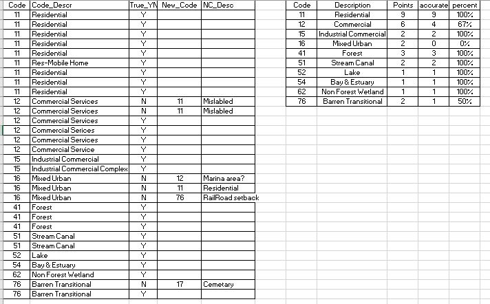
This week in lab we took our LULC map from last week and performed ground truth via Google Map.  I randomly selected 30 points in a grid fashion and then adjusted to account for each land type from the original map.  Each point was located and verified in google map for the location land use.  Here is a summary table of those results.

Of the 30 sample points 24 of them were classified correctly for an overall accuracy of 80%.  The smaller table above shows the accuracy broken out by classifications.  Mixed Urban had 0% correct.  Since I utilized this class for areas that I could not completely identify when classifying it is reasonable that with additional data the need for this classification would be eliminated.

Land Use Land Cover Classification

This week in lab we practiced our skills of recognizing features on the ground using a natural color aerial photograph.  We digitized an area of Pascagoula, MS, creating a land use/land cover map.  We identified the ground based on size, shape, color, pattern, shadows and association.  We utilized the USGS Standard Land Use / Land Cover Classification System.  The assignment was to categorize to level two (two digit classification).  Classifications of three or higher are typically utilized for local and some regional planning. 

My specific categories for this project 

Part of my employment background was working for 10 years in a building department in a municipality.  We worked very closely with the planning department and GIS guy.  Identifying urban land use from aerial perspectives I have done before.  It is a lot easier when you are familiar with the area.  Correctly identifying natural elements just at a level 2 classification was difficult because I am not familiar with the difference in kinds of trees or when a stream or canal becomes part of an estuary or bay. 

Technically doing the polygons was new and still somewhat challenging in the new to me GIS Pro.  My first attempt I did not have the Edge snapping or vertex snapping turned on, so I utilized this attempt as practice.  The second attempt I did turn on the snapping features while creating the polygons.  First creating a feature class file in my gdb.  Then in the edit tab clicking the create button and choosing polygon.  It was challenging to be able to navigate the picture while creating the polygon.  I settled on zooming in and out with the mouse scroll to move the image without having to click.  I did not master the clip portion to separate smaller interior polygons from larger surrounding areas.  Instead I relied on more of a lasso method with the larger polygon.  I started with larger easily identified areas keeping my attribute table open and adding the code as I drew each polygon (realizing that you must click off the cell in the attribute table that you are making changes to before you save the changes or that cell will not be recorded).  As I progressed from larger isolated polygons then I started working right and left back and forth to fill in the surrounding areas and smaller isolations.  Distinguishing between commercial service and commercial industrial was harder without knowledge of the practice of the location.  Ultimately, I settled on cleaner sites without outside materials or industrial roof or ground mechanisms and Commercial Service and those with as Commercial Industrial.

Visual Interpretation

This week in Photo Interpretation and Remote Sensing we  learned more about the types of and techniques for interpreting aerial photography. We were provided background on the types of aerial cameras, the different types of images they capture (oblique, vertical, stereo), the types of film used by traditional cameras, and understand how resolution (spatial, spectral, temporal) applies to aerial photography. We also learned concepts, techniques, and application of visually interpreting aerial photos. We learned about the methods and techniques used to visually interpret aerial photos (i.e. recognition elements). These techniques form the basis for deriving geographic features and/or land use land cover types from aerial photos and that are used in a wide variety of real world applications. 

In the laboratory exercise, we learned some basic principles of interpreting features found on aerial photographs.  The first map above illustrates ranges of tone and texture for this photo.  The second map above demonstrates examples of elements identified, at least partially, by shape and size, pattern, shadow, and association of the surroundings.  We also examined a true color image (blue, green, red), identifying 5 areas of color and compared those elements in the same image provided in false color (green, red, and infrared).

We have moved from ArcGIS desktop to ArcGIS Pro and it has been a disorienting week.  The changes are vast! location of symbology, labeling, and properties are different, but even the environment has changed to a project oriented system instead of .mdx maps.  I am sure I will catch up as soon as I figure out how to control drive location.  

Final Project: Plano, Texas Exploration

Project Proposal:  Plano, Texas Exploration for Hobbs’

 My final project is a location decision for Mr. and Mrs. Hobbs.  They moved to Plano, TX to retire in April to be closer to their daughter and her family.  They are unfamiliar with the area and have asked me, another daughter, to come up with some geographic information for them.  They have already found their new home but would like to get to know the area better.  They asked for locations of the hospitals, parks, airports, toll roads and any other information that would assist them in becoming acquainted to their new environment.  Locating amenities near the Hobbs’ will provide them with a much clearer picture of the area and help them feel more at home.  Maps and tables are provided to highlight areas like their home in relation to their daughters and the location of the toll roads, hospitals and airports.  Geocoding of farmers markets, museums and other destinations have been included.  GIS analysis of buffered and clipped data to utilize for euclidean distance and weighted overlay analysis has been performed to come up with some areas for the Hobbs' to explore based on their interests.

Final Project: Python

My final project proposal is to locate cities or towns in Texas of a minimum size (thinking 100,000) that are within 50 miles of a major airport that contain a lake or river.  I will need to obtain data for the state of Texas including lakes and rivers as well as airports and population of cities.  Utilizing python script: 1) create a buffer around airports of maybe 50 miles.  2)Clip population data and lake/river data to airport buffers.  3)utilize the results to Create a search cursor to locate cities or towns over 100,000 in population 4)print the list of locations.

First image above is of the printed list of cities/towns with populations over 100,000, that are within 50 miles of an airport and the second is of the printed dictionary containing the name of the city and the population.  Below is an image of the catalog files showing the Clipped cities and NHD in the results folder.

Module 11: Sharing Tools

The FINAL MODULE for GIS Programming!  We explored different methods for sharing script tools, learned ESRI recommended folder and file structure for sharing script tools, identified data and workspaces for script tools.  We learned  how to created a geoprocessing package, embed scripts and password protection tools and created script tool documentation.

This week in lab we focused on the standard folder structure and filepaths necessary when sharing tools and looked at some geoprocessing packages that provide an alternative solution to distributing script tools.