Module 6: Homeland Security: Minimum Essential Data Set Prepare

The Department of Homeland Security (DHS) Goal is: “A secure and resilient nation with the capabilities required across the whole community to prevent, protect against, mitigate, respond to, and recover from the threats and hazards that pose the greatest risk.”  The Homeland Security Infrastructure Program (HSIP) is a joint effort of National Geospatial-Intelligence Agency, USGS, and the Federal Geographic Data Committee, established the development of Minimum Essential Data Sets (MEDS) to conduct their missions in support of homeland defense and security.  The Minimum Essential Data Sets stipulated by DHS as minimal essential datasets are boundaries, orthoimagery, geographic names, transportation, land cover, elevations and hydrography. 

In this week's lab we prepared a geospatial dataset for homeland security planning and operations.  Prepare as defined by the Department of Homeland Security (DHS), as "the necessary action to put something into a state where it is fit for use or action, or for particular event of purpose.  We were provided data download transportation, national hydrography, landmark data, orthoimagery, elevation, and geographic names data from the National Map Viewer.  We created comprehensive and interoperable geospatial database.  We identify the Minimum Essential Dataset stipulated by DHS.  We manipulate and query spatial data using geoprocessing tools, explore data frame and layer projection properties and join tables to categorize feature classes.  We added a color map to layer symbology, convert text and x,y data to feature class, and save group layers as layer files.  We did all of this to prepare GIS data for analysis.

Module 5: Homeland Security: Washington DC Crime Mapping

This week we moved into utilizing GIS to benefit law enforcement. 

Law enforcement agencies daily responsibility of protecting life and property while keeping the peace in their communities:  responding to crime reports, investigating criminal activities to apprehend those responsible, thwarting would be criminal activities, monitoring known criminals 

GIS provides a visual, spatial means of displaying data, allowing law enforcement agencies to make informed decisions more quickly.  GIS can assist law enforcement with by helping to identify an incident location, generate a location report, visualize an incident location, analyze an impacted area and coordinate resources.  

Crime Analysis is the qualitative and quantitative study of crime and police related information in combination with socio-demographic and spatial factors.  The primary goals of crime analysis are to apprehend criminals, prevent crime, reduce disorder, and evaluate organizational procedures.

In lab this week we establish workspace environments (view-data frame properties-coordinate system) and tool environments (right click in the toolbox menu, outside of a tool, select environments-expand workspace-set current workspace, output coordinate system set to same as display, for processing extent set to same as Washington DC layer, raster analysis setting set raster cell size to 73, set the mask to Washington DC).  We utilized Address Locator to create points for the police stations and added points by hand for the 3 unmatched addresses by utilizing google map to obtain the location.  We added a filed to attribute table and utilized the field calculator and entered the formula.  We utilized the multi ring buffer tool to set buffers around police stations.  We joined layers based on spatial location.  We utilized kernel density tool from spatial analyst toolset to create crime densities for burglaries, homicides and sex abuse crimes.  

The first map has a TON of information - much more than I would have thought possible:

• population density choropleth by census block group
• location of police stations with graduated symbols showing percent of crimes being handled in that station
• 3 ring police station buffer transparency overlay
• points of the crimes
• Summary Graph showing the count by type of crimes
• Each station is labeled with the name and percent of total crimes that station handeled
• Proposed location of a new station based on station buffers, crimes, and neighboring station percent of crimes.

The second map has 3 data frames that show the results of the kernel density for burglaries, homicides and sex abuse crimes.  Each of the density results is shown as a transparency over the population density choropleth.  The neighboring results allow for comparison of each crimes hotspots.

Module 6: Geoprocessing with Python

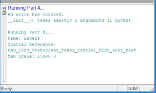
Above is the messages from the script I wrote and ran this week.  I utilized Model Builder in ArcGIS to get the basic code and then exported it to a python script and edited in PythonWin.  The instructions for the assignment were to write a script that performs the three geo-processing functions: Add XY tool, Buffer tool, and Dissolve tool. Get Message function was utilized following each tool to document the successful completion of each tool.

ArcPy site package is like a library of functions that add functionality to Python.  The site package works very much like a module, but a package contains multiple modules as well as functions and classes. 

A function in Python is a specific bit of program that does a specific task. Functions syntax is typically: <function>(<arguments>)

A method is a function that is closely coupled to an object.  Method is called as follows: <object>.<method>(<arguments>)

Classes can be used to create objects, and once the object is created, its properties and methods can be used.  Classes are often used to avoid having to use long and complicated strings.  Arcpy classes are often used as shortcuts for tool parameters that would otherwise have a more complicated equivalent.  Syntax for setting the property of a class is:  <classname>.<property>=<value>

Tools can be called 1)by its function- arcpy.<toolname_toolboxalias>(<parameters>) or 2) as a module- arcpy.<toolboxalias>.<toolname>(<parameters>) 3)once a particular tool is identified, the tool's syntax can be accessed from python using the Usage function
All tools are functions, but not all functions are tools. 

One of the points from our exercises for this week was a focus on getting help with syntax.  Help with syntax can be obtained a number of ways.  A couple of ways are: 1) help panel is visible within the Python window, entering the code brings up the syntax for the tool 2)from the search menu, search the tool, clicking the definition in the search tool will bring up the item description that contains syntax and examples of code.

Module 5: GeoProcessing

This week the focus was geoprocessing.  Geoprocessing in its most basic form is a series of actions performed on geographic data.  There are many geo processes, including reprojections, clipping and buffering.   Central to the concept is that there is input data (one-or-more), the process/task itself and then the output data.

There are two categories of tools:  1)System: These include the built-in types of tools or of any type that are created by Esri. These tools themselves are not run in sequence, but can
be run in batch mode and 2)Custom: Tools of any type that can be built by a user or obtained from
third-party developers. And these are the type that we are learning to begin building in this class.

There are also types of tools:  1)Built-in: The tools that come w/ the Esri installation as part of ArcGIS are known of as the built-in tools. These tools are created with programming languages such as c++ and the .net languages,  2)Model: built using ModelBuilder, and 3)Script: Tools that run a script through a tool interface

The four elements of models are 1)project data (input) 2)tool (process) 3)derived data (output) 4)connectors (arrows to show the direction of data flow).

We also set our current workspace, in environments, to your specific module results folder and set the scratch workspace, where temporary files and folders are housed. 

ArcGIS tools have python script behind the scenes and as such can be exported from a model to a python script.  However the script that is exported is typically not a stand alone script.  To become a stand alone script, the exported script could need additional information, like lines of code and/or full drive addresses for data locations.

In this week's lab we practiced several types of geoprocessing, including batch processing (running a tool or series of tools on multiple inputs, set the parameters once and list inputs, processing time is the same but the set up time is saved) , making new tools with ModelBuilder, and converting models into scripts and script tools. We created our own model and script tools that perform two simple geoprocessing tasks (clip, select and erase). The results are the picture above.  Finally, we shared our toolbox with the dropbox submission.  

Module 4: Hurricanes

This week in lab we focused on hurricanes.  We learned about different hurricane categories in the Saffir Simpson Scale, forms of hurricane hazard, hurricane terminology, and identified key GIS tools used in damage assessment.  We examined hurricane tracking points in Microsoft Excel Database, displayed those points using xy tool, created data using points to line feature to get the path of the hurricane from the tracking points, explored marker symbol options and utilized the hurricane symbol, created a VB script for labeling allowing each point to label two variables (wind speed and pressure), preformed two raster mosaics, tried to explore Effects Toolbar, added damage points and defined damage, generated table on damage results.  

I was unsuccessful getting the Effects Toolbar to cooperate, several of my buttons were greyed out.  Still investigating a solution.  I was able to compare pre and post storm images by having them on top of each other in the data frame and turning on layer on and off while I observed the changes.

Module 4: GIS Programing

Above are the results of the scripts this week.  This week we learned to recognize syntax errors and exceptions, syntax errors show up when the script is checked, exceptions are not caught by a check of the script but will result in an error message when the script is run.  We practiced using debugging by stepping through code, adding print statements to check progress in a script, commenting out code to skip parts and we "caught" "thrown" exception errors with try-except statements.  We also learned that syntax errors are errors with the way the script is written, and that logical errors do not affect the syntax so for this lab they were spelling errors and file location errors.  

Peer Review: Scripting MODFLOW

Review of Scripting MODFLOW Model Development Using Python and FloPy

The overall organization of the paper was good.  Sections for Abstract, Introduction, Conclusion, Acknowledgments and References were all present and clearly labeled.  The material was ordered so that it is logical.  Subheadings helped to break up the main arguments into a basic example, advantages of scripting, and a more complex example.

The introduction of the paper gave a clear purpose of the paper, utilizing python script as alternative to utilizing GUI (graphical user interface) for the construction of a groundwater model. Historical use of a GUI in groundwater modeling is reported concisely.  Adequate citation is provided throughout the introduction.  The conclusion of the introduction clearly states the position of the paper as well as well as potential oppositions to be addressed.

The methods and results although sometimes outside the scope of my understanding appear to be adequate in detail and explanation.

The conclusion section opens the discussion of how the use of python programing instead of GUI facilitates analyses that can be difficult of impossible to complete with GUI, automating processing, records steps making it reproducibly by others, all while utilizing open source language (Python) and open source tools (FloPy).

Acknowledgments are generally given to contributors.  Welcome for additional information and or suggestions.  Standard non-endorsement statement included.

References appear to be in ample supply as well as well sited and organized.

References

Bakker, M., Post, V., Langevin, C.D., Hughes, J.D., White, J.T., Starn, J.J., & Fiennen, M.N. (2106, March 30).  Scripting MODFLOW Model Development Using Python and FloPy, Groundwater, 54: 733-739.  https://doi.org/10.1111/gwat.12413

Scripting MODFLOW Model Development Using Python and FloPY

Module 3: Tsunamis

This week we examined Tsunamis.  Tsunamis are basically a series of waves that occur as a result of a large water displacement.  The displacement can be caused by an underwater earthquake or landslide.  The water displacement moves like dropping a pebble in a body of water, ripples moving away from the site of displacement.  Runup is the term utilized for the waves pushing up on land and through rivers and streams.  Disaster response to this type of even includes assessing hazard situations like contaminations and fires, property damage including public and private, people evacuations, sites for evacuees, equipping those sites with water, food, and medicine.  GIS can be utilized to show extent of damage, potential sites for evacuees, what services are needed in what area and how to get them there. 

This week in lab we worked with information relevant to response and recovery efforts of the Japan Tsunami.  Set up a geodatabase with file geodatabase to help organize data by category utilizing feature.  Mosaicked raster and built raster attribute data.  Utilized the multi-ring buffer and clip tool to create evacuation zones for the Nuclear Power Plant.  Analyze runup on the coast and created 3 evacuation zones.  Created an expression to label features by two fields (name and population of cities).  Utilize ModelBuilding with elevation data to automate the evacuation zone mapping.   

Module 3: Python Fundamentals Part 2

This week we studied more advanced aspects of Python scripting.  We learned correct usage of file paths, how to import modules for additional functions, appropriate naming conventions, loop structures, and commenting.  We examined conditional statements that perform different actions in different situations, and for and while loops that repeat the same processes multiple times. We also practiced finding and fixing errors in Python code.  In this week's lab we were asked to use modules to access a wider range of methods and functions, write conditional statements and loop structures, and identify and correct errors in code.
The lab assignment, was to complete an unfinished Python script, correcting some errors in it, and adding new blocks of code. The result if successful would have been a complete Python script, including a comments section containing your name and contact information, the date the script was completed, and a brief description of its purpose. 

At the due date, Wednesday, I have not been successful. 

Thursday: attended virtual office hours with professor, made progress past sticking point.  Only to encounter another sticking point.

Friday: requested email assistance from professor.  Finally completed module successfully.

Hope these struggles are not indicative of the rest of the semester!  Need my brain to learn to think in python.

Mod 2: Lahars

This week in Applications of GIS we learned terms associated with disaster management:  natural hazard, risk, and mitigation.  We identified some strategies to utilize GIS to help manage hazards.  We looked at ways GIS is utilized to identify areas of concern and areas of public concern.  We identified features at risk during a lahar event (population, schools, infrastructure).  We mosaicked two Digital Elevation Models (DEM) to obtain a single layer.  We predict possible inundation zones from a lahar event from Mount Hood in Oregon.  We created the point for Mount Hood utilizing the XY tool and converted it to a graphic feature.  Predictions were made by utilizing ArcMap spatial analyst Hydrology tools on DEM to create a Fill raster to remove small imperfections, Flow raster to represent the direction across each cell, and Flow Accumulation raster to show which cells receive the most flow.  We utilized Raster Math to change the raster from float point data (continuous) to integer data, calculated 1% of total pixels to perform Stream Classification, Con Tool to limit the stream calculation to greater than 1% of the total pixels and finally hydrology tool Stream to Feature to obtain a polyline vector feature to utilize in the Lahar's Analysis map from above.  Census block groups were selected that intersected a 1/2 mile buffered Stream that allowed for population in those block groups.  Locations of schools within the 1/2 mile buffered Stream were also mapped.